
Intro
Learn Excel conditional formatting dates techniques to highlight specific date ranges, overdue dates, and upcoming events using formulas, rules, and formatting options.
When working with dates in Excel, it's often useful to highlight cells based on specific conditions, such as dates within a certain range, dates that are overdue, or dates that are upcoming. Excel's Conditional Formatting feature makes it easy to apply formatting to cells based on these conditions. In this article, we'll explore how to use Conditional Formatting to highlight dates in Excel.
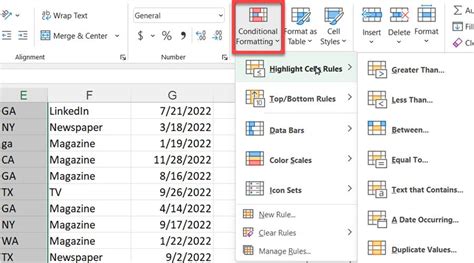
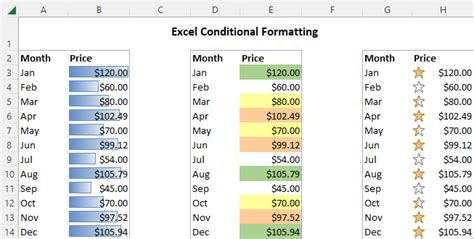
Conditional Formatting is a powerful tool that allows you to apply formatting to cells based on specific conditions. You can use it to highlight cells that contain certain values, dates, or formulas. To access Conditional Formatting, select the cells you want to format, go to the Home tab, and click on the Conditional Formatting button in the Styles group.
Highlighting Dates within a Specific Range
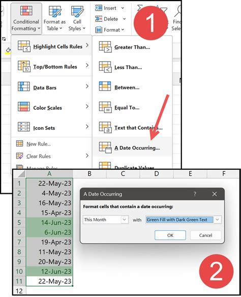
To highlight dates within a specific range, you can use the "Date Occurring" rule in Conditional Formatting. For example, suppose you have a list of dates in column A, and you want to highlight all dates that occur within the next 30 days. To do this, select the cells in column A, go to the Home tab, click on Conditional Formatting, and select "New Rule." Then, choose "Use a formula to determine which cells to format," and enter the following formula: =TODAY()+30>=A1. This formula checks if the date in cell A1 is within the next 30 days. If the formula is true, the cell will be formatted.
Using Formulas with Conditional Formatting
You can use a variety of formulas with Conditional Formatting to highlight dates based on specific conditions. For example, you can use the `TODAY()` function to highlight dates that are overdue or upcoming. You can also use the `WEEKDAY()` function to highlight dates that fall on specific days of the week.Highlighting Overdue Dates
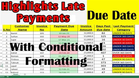
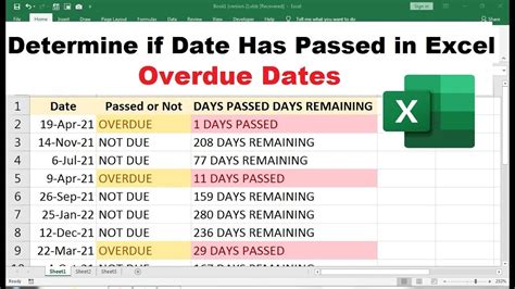
To highlight overdue dates, you can use the "Date Occurring" rule in Conditional Formatting. For example, suppose you have a list of dates in column A, and you want to highlight all dates that are overdue. To do this, select the cells in column A, go to the Home tab, click on Conditional Formatting, and select "New Rule." Then, choose "Use a formula to determine which cells to format," and enter the following formula: =A1<TODAY(). This formula checks if the date in cell A1 is before the current date. If the formula is true, the cell will be formatted.
Using Multiple Conditions with Conditional Formatting
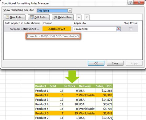
You can use multiple conditions with Conditional Formatting to highlight dates based on specific conditions. For example, you can use the `AND()` function to highlight dates that meet two or more conditions. You can also use the `OR()` function to highlight dates that meet one or more conditions.Highlighting Upcoming Dates
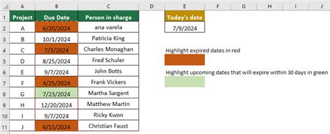
To highlight upcoming dates, you can use the "Date Occurring" rule in Conditional Formatting. For example, suppose you have a list of dates in column A, and you want to highlight all dates that are within the next 7 days. To do this, select the cells in column A, go to the Home tab, click on Conditional Formatting, and select "New Rule." Then, choose "Use a formula to determine which cells to format," and enter the following formula: =TODAY()+7>=A1. This formula checks if the date in cell A1 is within the next 7 days. If the formula is true, the cell will be formatted.
Using Conditional Formatting with Other Excel Functions
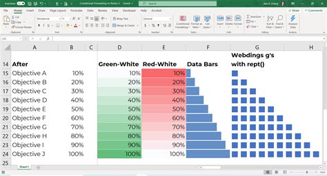
You can use Conditional Formatting with other Excel functions, such as filtering and sorting, to analyze and visualize your data. For example, you can use the `FILTER()` function to filter your data based on specific conditions, and then use Conditional Formatting to highlight the filtered data.Best Practices for Using Conditional Formatting

Here are some best practices to keep in mind when using Conditional Formatting:
- Use clear and concise formulas to determine which cells to format.
- Use multiple conditions to highlight dates based on specific conditions.
- Use the
AND()andOR()functions to combine multiple conditions. - Use Conditional Formatting with other Excel functions, such as filtering and sorting, to analyze and visualize your data.
- Use the
TODAY()function to highlight dates that are overdue or upcoming.
Common Mistakes to Avoid
Here are some common mistakes to avoid when using Conditional Formatting: * Using unclear or ambiguous formulas to determine which cells to format. * Not using multiple conditions to highlight dates based on specific conditions. * Not using the `AND()` and `OR()` functions to combine multiple conditions. * Not using Conditional Formatting with other Excel functions, such as filtering and sorting, to analyze and visualize your data.Conditional Formatting Image Gallery


What is Conditional Formatting in Excel?
+Conditional Formatting is a feature in Excel that allows you to apply formatting to cells based on specific conditions.
How do I use Conditional Formatting to highlight dates?
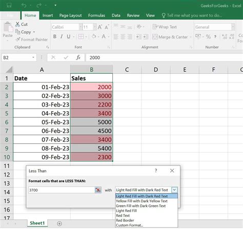
+To use Conditional Formatting to highlight dates, select the cells you want to format, go to the Home tab, click on Conditional Formatting, and select "New Rule." Then, choose "Use a formula to determine which cells to format," and enter a formula that checks if the date meets the condition you want to highlight.
Can I use multiple conditions with Conditional Formatting?
+Yes, you can use multiple conditions with Conditional Formatting by using the `AND()` and `OR()` functions to combine multiple conditions.
How do I use the `TODAY()` function with Conditional Formatting?
+To use the `TODAY()` function with Conditional Formatting, enter a formula that checks if the date is within a certain range of the current date. For example, `=TODAY()+7>=A1` checks if the date in cell A1 is within the next 7 days.
What are some best practices for using Conditional Formatting?
+Some best practices for using Conditional Formatting include using clear and concise formulas, using multiple conditions, and using the `AND()` and `OR()` functions to combine multiple conditions.
In summary, Conditional Formatting is a powerful tool in Excel that allows you to apply formatting to cells based on specific conditions. By using formulas and multiple conditions, you can highlight dates that meet certain criteria, such as dates within a specific range, overdue dates, or upcoming dates. By following best practices and using Conditional Formatting with other Excel functions, you can analyze and visualize your data more effectively. If you have any questions or need further assistance, don't hesitate to ask. Share your experiences with Conditional Formatting in the comments below, and feel free to share this article with others who may find it helpful.